

Python如何利用GDAL模块实现读取栅格数据并对指定数据加以筛选掩膜
1代码分段讲解1.1模块与路径准备首先,需要对用到的模块与存放栅格图像的各类路径加以准备。importosimportcopyimportnumpyasnpimportpylabaspltfromosgeoimportgdal#rt_file_path="G:/Postgraduate/LAI_Glass_RTlab/Rc_Lai_A2018161_h22v03.tif"#gl_file_path="G:/Postgraduate/LAI_Glass_RTlab/GLASS01E01.V50.A20181
1 代码分段讲解
1.1 模块与路径准备
首先,需要对用到的模块与存放栅格图像的各类路径加以准备。
import os
import copy
import numpy as np
import pylab as plt
from osgeo import gdal

# rt_file_path="G:/Postgraduate/LAI_Glass_RTlab/Rc_Lai_A2018161_h22v03.tif"
# gl_file_path="G:/Postgraduate/LAI_Glass_RTlab/GLASS01E01.V50.A2018161.h22v03.2020323.hdf"
# out_file_path="G:/Postgraduate/LAI_Glass_RTlab/test.tif"
rt_file_path="I:/LAI_RTLab/A2018161/"
gl_file_path="I:/LAI_Glass/2018161/"
out_file_path="I:/LAI_Dif/"
其中,rt_file_path为自有产品的存放路径,gl_file_path为GLASS产品的存放路径,out_file_path为最终二者栅格做完差值处理后结果的存放路径。
1.2 栅格图像文件名读取与配对
接下来,需要将全部待处理的栅格图像用os.listdir()进行获取,并用for循环进行循环批量处理操作的准备。
rt_file_list=os.listdir(rt_file_path)
for rt_file in rt_file_list:
    file_name_split=rt_file.split("_")
    rt_hv=file_name_split[3][:-4]

    gl_file_list=os.listdir(gl_file_path)
    for gl_file in gl_file_list:
        if rt_hv in gl_file:
            rt_file_tif_path=rt_file_path+rt_file
gl_file_tif_path=gl_file_path+gl_file其中,由于本文需求是对两种产品做差,因此首先需要结合二者的hv分幅编号,将同一分幅编号的两景遥感影像放在一起;因此,依据自有产品文件名的特征,选择.split()进行字符串分割,并随后截取获得遥感影像的hv分幅编号。
1.3 输出文件名称准备
前述1.1部分已经配置好了输出文件存放的路径,但是还没有进行输出文件文件名的配置;因此这里我们需要配置好每一个做差后的遥感影像的文件存放路径与名称。其中,我们就直接以遥感影像的hv编号作为输出结果文件名。
            DRT_out_file_path=out_file_path+"DRT/"
            if not os.path.exists(DRT_out_file_path):
                os.makedirs(DRT_out_file_path)
            DRT_out_file_tif_path=os.path.join(DRT_out_file_path,rt_hv+".tif")

            eco_out_file_path=out_file_path+"eco/"
            if not os.path.exists(eco_out_file_path):
                os.makedirs(eco_out_file_path)
            eco_out_file_tif_path=os.path.join(eco_out_file_path,rt_hv+".tif")

            wat_out_file_path=out_file_path+"wat/"
            if not os.path.exists(wat_out_file_path):
                os.makedirs(wat_out_file_path)
            wat_out_file_tif_path=os.path.join(wat_out_file_path,rt_hv+".tif")

            tim_out_file_path=out_file_path+"tim/"
            if not os.path.exists(tim_out_file_path):
                os.makedirs(tim_out_file_path)
            tim_out_file_tif_path=os.path.join(tim_out_file_path,rt_hv+".tif")
这一部分代码分为了四个部分,是因为自有产品的LAI是分别依据四种算法得到的,在做差时需要每一种算法分别和GLASS产品进行相减,因此配置了四个输出路径文件夹。
1.4 栅格文件数据与信息读取
接下来,利用gdal模块对.tif与.hdf等两种栅格图像加以读取。
            rt_raster=gdal.Open(rt_file_path+rt_file)
            rt_band_num=rt_raster.RasterCount
            rt_raster_array=rt_raster.ReadAsArray()
            rt_lai_array=rt_raster_array[0]
            rt_qa_array=rt_raster_array[1]
            rt_lai_band=rt_raster.GetRasterBand(1)
            # rt_lai_nodata=rt_lai_band.GetNoDataValue()
            # rt_lai_nodata=32767
            # rt_lai_mask=np.ma.masked_equal(rt_lai_array,rt_lai_nodata)
            rt_lai_array_mask=np.where(rt_lai_array>30000,np.nan,rt_lai_array)
            rt_lai_array_fin=rt_lai_array_mask*0.001

            gl_raster=gdal.Open(gl_file_path+gl_file)
            gl_band_num=gl_raster.RasterCount
            gl_raster_array=gl_raster.ReadAsArray()
            gl_lai_array=gl_raster_array
            gl_lai_band=gl_raster.GetRasterBand(1)
            gl_lai_array_mask=np.where(gl_lai_array>1000,np.nan,gl_lai_array)
            gl_lai_array_fin=gl_lai_array_mask*0.01

            row=rt_raster.RasterYSize
            col=rt_raster.RasterXSize
            geotransform=rt_raster.GetGeoTransform()
            projection=rt_raster.GetProjection()
首先,以上述代码的第一段为例进行讲解。其中,gdal.Open()读取栅格图像;.RasterCount获取栅格图像波段数量;.ReadAsArray()将栅格图像各波段的信息读取为Array格式,当波段数量大于1时,其共有三维,第一维为波段的个数;rt_raster_array[0]表示取Array中的第一个波段,在本文中也就是自有产品的LAI波段;rt_qa_array=rt_raster_array[1]则表示取出第二个波段,在本文中也就是自有产品的QA波段;.GetRasterBand(1)表示获取栅格图像中的第一个波段(注意,这里序号不是从0开始而是从1开始);np.where(rt_lai_array>30000,np.nan,rt_lai_array)表示利用np.where()函数对Array中第一个波段中像素>30000加以选取,并将其设置为nan,其他值不变。这一步骤是消除图像中填充值、Nodata值的方法。最后一句*0.001是将图层原有的缩放系数复原。
其次,上述代码第三段为获取栅格行、列数与投影变换信息。
1.5 差值计算与QA波段筛选
接下来,首先对自有产品与GLASS产品加以做差操作,随后需要对四种算法分别加以提取。
            lai_dif=rt_lai_array_fin-gl_lai_array_fin
            lai_dif=lai_dif*1000

            rt_qa_array_bin=copy.copy(rt_qa_array)
            rt_qa_array_row,rt_qa_array_col=rt_qa_array.shape
            for i in range(rt_qa_array_row):
                for j in range(rt_qa_array_col):
                    rt_qa_array_bin[i][j]="{:012b}".format(rt_qa_array_bin[i][j])[-4:]

            # DRT_pixel_pos=np.where((rt_qa_array_bin>=100) & (rt_qa_array_bin==11))
            # eco_pixel_pos=np.where((rt_qa_array_bin<100) & (rt_qa_array_bin==111))
            # wat_pixel_pos=np.where((rt_qa_array_bin<1000) & (rt_qa_array_bin==1011))
            # tim_pixel_pos=np.where((rt_qa_array_bin<1100) & (rt_qa_array_bin==1111))

            # colormap=plt.cm.Greens
            # plt.figure(1)
            # # plt.subplot(2,4,1)
            # plt.imshow(rt_lai_array_fin,cmap=colormap,interpolation='none')
            # plt.title("RT_LAI")
            # plt.colorbar()
            # plt.figure(2)
            # # plt.subplot(2,4,2)
            # plt.imshow(gl_lai_array_fin,cmap=colormap,interpolation='none')
            # plt.title("GLASS_LAI")
            # plt.colorbar()
            # plt.figure(3)
            # dif_colormap=plt.cm.get_cmap("Spectral")
            # plt.imshow(lai_dif,cmap=dif_colormap,interpolation='none')
            # plt.title("Difference_LAI (RT-GLASS)")
            # plt.colorbar()

            DRT_lai_dif_array=np.where((rt_qa_array_bin>=100) | (rt_qa_array_bin==11),
                                       np.nan,lai_dif)
            eco_lai_dif_array=np.where((rt_qa_array_bin<100) | (rt_qa_array_bin==111),
                                       np.nan,lai_dif)
            wat_lai_dif_array=np.where((rt_qa_array_bin<1000) | (rt_qa_array_bin==1011),
                                       np.nan,lai_dif)
            tim_lai_dif_array=np.where((rt_qa_array_bin<1100) | (rt_qa_array_bin==1111),
                                       np.nan,lai_dif)

            # plt.figure(4)
            # plt.imshow(DRT_lai_dif_array)
            # plt.colorbar()
            # plt.figure(5)
            # plt.imshow(eco_lai_dif_array)
            # plt.colorbar()
            # plt.figure(6)
            # plt.imshow(wat_lai_dif_array)
            # plt.colorbar()
            # plt.figure(7)
            # plt.imshow(tim_lai_dif_array)
            # plt.colorbar()
其中,上述代码前两句为差值计算与数据化整。将数据转换为整数,可以减少结果数据图层的数据量(因为不需要存储小数了)。
随后,开始依据QA波段进行数据筛选与掩膜。其实各类遥感影像(例如MODIS、Landsat等)的QA波段都是比较近似的:通过一串二进制码来表示遥感影像的质量、信息等,其中不同的比特位往往都代表着一种特性。例如下图所示为Landsat Collection 2 Level-2的QA波段含义。
在这里,QA波段原本为十进制(一般遥感影像为了节省空间,QA波段都是写成十进制的形式),因此需要将其转换为二进制;随后通过获取指定需要的二进制数据位数(在本文中也就是能确定自有产品中这一像素来自于哪一种算法的二进制位数),从而判断这一像素所得LAI是通过哪一种算法得到的,从而将每种算法对应的像素分别放在一起处理。DRT_lai_dif_array等四个变量分别表示四种算法中,除了自己这一种算法得到的像素之外的其他所有像素;之所以选择这种方式,是因为后期我们可以将其直接掩膜掉,那么剩下的就是这种算法自身的像素了。
其中,上述代码注释掉的plt相关内容可以实现绘制空间分布图,大家感兴趣可以尝试使用。
1.6 结果栅格文件写入与保存
接下来,将我们完成上述差值计算与依据算法进行筛选后的图像保存。
            driver=gdal.GetDriverByName("Gtiff")
            out_DRT_lai=driver.Create(DRT_out_file_tif_path,row,col,1,gdal.GDT_Float32)
            out_DRT_lai.SetGeoTransform(geotransform)
            out_DRT_lai.SetProjection(projection)
            out_DRT_lai.GetRasterBand(1).WriteArray(DRT_lai_dif_array)
            out_DRT_lai=None

            driver=gdal.GetDriverByName("Gtiff")
            out_eco_lai=driver.Create(eco_out_file_tif_path,row,col,1,gdal.GDT_Float32)
            out_eco_lai.SetGeoTransform(geotransform)
            out_eco_lai.SetProjection(projection)
            out_eco_lai.GetRasterBand(1).WriteArray(eco_lai_dif_array)
            out_eco_lai=None

            driver=gdal.GetDriverByName("Gtiff")
            out_wat_lai=driver.Create(wat_out_file_tif_path,row,col,1,gdal.GDT_Float32)
            out_wat_lai.SetGeoTransform(geotransform)
            out_wat_lai.SetProjection(projection)
            out_wat_lai.GetRasterBand(1).WriteArray(wat_lai_dif_array)
            out_wat_lai=None

            driver=gdal.GetDriverByName("Gtiff")
            out_tim_lai=driver.Create(tim_out_file_tif_path,row,col,1,gdal.GDT_Float32)
            out_tim_lai.SetGeoTransform(geotransform)
            out_tim_lai.SetProjection(projection)
            out_tim_lai.GetRasterBand(1).WriteArray(tim_lai_dif_array)
            out_tim_lai=None

print(rt_hv)其中,.GetDriverByName("Gtiff")表示保存为.tif格式的GeoTIFF文件;driver.Create(DRT_out_file_tif_path,row,col,1,gdal.GDT_Float32)表示按照路径、行列数、波段数与数据格式等建立一个新的栅格图层,作为输出图层的框架;其后表示分别将地理投影转换信息与像素具体数值分别赋予这一新建的栅格图层;最后=None表示将其从内存空间中释放,完成写入与保存工作。
2 完整代码
本文所需完整代码如下:
# -*- coding: utf-8 -*-
"""
Created on Thu Jul 15 19:36:15 2021

@author: fkxxgis
"""

import os
import copy
import numpy as np
import pylab as plt
from osgeo import gdal

# rt_file_path="G:/Postgraduate/LAI_Glass_RTlab/Rc_Lai_A2018161_h22v03.tif"
# gl_file_path="G:/Postgraduate/LAI_Glass_RTlab/GLASS01E01.V50.A2018161.h22v03.2020323.hdf"
# out_file_path="G:/Postgraduate/LAI_Glass_RTlab/test.tif"
rt_file_path="I:/LAI_RTLab/A2018161/"
gl_file_path="I:/LAI_Glass/2018161/"
out_file_path="I:/LAI_Dif/"

rt_file_list=os.listdir(rt_file_path)
for rt_file in rt_file_list:
    file_name_split=rt_file.split("_")
    rt_hv=file_name_split[3][:-4]

    gl_file_list=os.listdir(gl_file_path)
    for gl_file in gl_file_list:
        if rt_hv in gl_file:
            rt_file_tif_path=rt_file_path+rt_file
            gl_file_tif_path=gl_file_path+gl_file

            DRT_out_file_path=out_file_path+"DRT/"
            if not os.path.exists(DRT_out_file_path):
                os.makedirs(DRT_out_file_path)
            DRT_out_file_tif_path=os.path.join(DRT_out_file_path,rt_hv+".tif")

            eco_out_file_path=out_file_path+"eco/"
            if not os.path.exists(eco_out_file_path):
                os.makedirs(eco_out_file_path)
            eco_out_file_tif_path=os.path.join(eco_out_file_path,rt_hv+".tif")

            wat_out_file_path=out_file_path+"wat/"
            if not os.path.exists(wat_out_file_path):
                os.makedirs(wat_out_file_path)
            wat_out_file_tif_path=os.path.join(wat_out_file_path,rt_hv+".tif")

            tim_out_file_path=out_file_path+"tim/"
            if not os.path.exists(tim_out_file_path):
                os.makedirs(tim_out_file_path)
            tim_out_file_tif_path=os.path.join(tim_out_file_path,rt_hv+".tif")

            rt_raster=gdal.Open(rt_file_path+rt_file)
            rt_band_num=rt_raster.RasterCount
            rt_raster_array=rt_raster.ReadAsArray()
            rt_lai_array=rt_raster_array[0]
            rt_qa_array=rt_raster_array[1]
            rt_lai_band=rt_raster.GetRasterBand(1)
            # rt_lai_nodata=rt_lai_band.GetNoDataValue()
            # rt_lai_nodata=32767
            # rt_lai_mask=np.ma.masked_equal(rt_lai_array,rt_lai_nodata)
            rt_lai_array_mask=np.where(rt_lai_array>30000,np.nan,rt_lai_array)
            rt_lai_array_fin=rt_lai_array_mask*0.001

            gl_raster=gdal.Open(gl_file_path+gl_file)
            gl_band_num=gl_raster.RasterCount
            gl_raster_array=gl_raster.ReadAsArray()
            gl_lai_array=gl_raster_array
            gl_lai_band=gl_raster.GetRasterBand(1)
            gl_lai_array_mask=np.where(gl_lai_array>1000,np.nan,gl_lai_array)
            gl_lai_array_fin=gl_lai_array_mask*0.01

            row=rt_raster.RasterYSize
            col=rt_raster.RasterXSize
            geotransform=rt_raster.GetGeoTransform()
            projection=rt_raster.GetProjection()

            lai_dif=rt_lai_array_fin-gl_lai_array_fin
            lai_dif=lai_dif*1000

            rt_qa_array_bin=copy.copy(rt_qa_array)
            rt_qa_array_row,rt_qa_array_col=rt_qa_array.shape
            for i in range(rt_qa_array_row):
                for j in range(rt_qa_array_col):
                    rt_qa_array_bin[i][j]="{:012b}".format(rt_qa_array_bin[i][j])[-4:]

            # DRT_pixel_pos=np.where((rt_qa_array_bin>=100) & (rt_qa_array_bin==11))
            # eco_pixel_pos=np.where((rt_qa_array_bin<100) & (rt_qa_array_bin==111))
            # wat_pixel_pos=np.where((rt_qa_array_bin<1000) & (rt_qa_array_bin==1011))
            # tim_pixel_pos=np.where((rt_qa_array_bin<1100) & (rt_qa_array_bin==1111))

            # colormap=plt.cm.Greens
            # plt.figure(1)
            # # plt.subplot(2,4,1)
            # plt.imshow(rt_lai_array_fin,cmap=colormap,interpolation='none')
            # plt.title("RT_LAI")
            # plt.colorbar()
            # plt.figure(2)
            # # plt.subplot(2,4,2)
            # plt.imshow(gl_lai_array_fin,cmap=colormap,interpolation='none')
            # plt.title("GLASS_LAI")
            # plt.colorbar()
            # plt.figure(3)
            # dif_colormap=plt.cm.get_cmap("Spectral")
            # plt.imshow(lai_dif,cmap=dif_colormap,interpolation='none')
            # plt.title("Difference_LAI (RT-GLASS)")
            # plt.colorbar()

            DRT_lai_dif_array=np.where((rt_qa_array_bin>=100) | (rt_qa_array_bin==11),
                                       np.nan,lai_dif)
            eco_lai_dif_array=np.where((rt_qa_array_bin<100) | (rt_qa_array_bin==111),
                                       np.nan,lai_dif)
            wat_lai_dif_array=np.where((rt_qa_array_bin<1000) | (rt_qa_array_bin==1011),
                                       np.nan,lai_dif)
            tim_lai_dif_array=np.where((rt_qa_array_bin<1100) | (rt_qa_array_bin==1111),
                                       np.nan,lai_dif)

            # plt.figure(4)
            # plt.imshow(DRT_lai_dif_array)
            # plt.colorbar()
            # plt.figure(5)
            # plt.imshow(eco_lai_dif_array)
            # plt.colorbar()
            # plt.figure(6)
            # plt.imshow(wat_lai_dif_array)
            # plt.colorbar()
            # plt.figure(7)
            # plt.imshow(tim_lai_dif_array)
            # plt.colorbar()

            driver=gdal.GetDriverByName("Gtiff")
            out_DRT_lai=driver.Create(DRT_out_file_tif_path,row,col,1,gdal.GDT_Float32)
            out_DRT_lai.SetGeoTransform(geotransform)
            out_DRT_lai.SetProjection(projection)
            out_DRT_lai.GetRasterBand(1).WriteArray(DRT_lai_dif_array)
            out_DRT_lai=None

            driver=gdal.GetDriverByName("Gtiff")
            out_eco_lai=driver.Create(eco_out_file_tif_path,row,col,1,gdal.GDT_Float32)
            out_eco_lai.SetGeoTransform(geotransform)
            out_eco_lai.SetProjection(projection)
            out_eco_lai.GetRasterBand(1).WriteArray(eco_lai_dif_array)
            out_eco_lai=None

            driver=gdal.GetDriverByName("Gtiff")
            out_wat_lai=driver.Create(wat_out_file_tif_path,row,col,1,gdal.GDT_Float32)
            out_wat_lai.SetGeoTransform(geotransform)
            out_wat_lai.SetProjection(projection)
            out_wat_lai.GetRasterBand(1).WriteArray(wat_lai_dif_array)
            out_wat_lai=None

            driver=gdal.GetDriverByName("Gtiff")
            out_tim_lai=driver.Create(tim_out_file_tif_path,row,col,1,gdal.GDT_Float32)
            out_tim_lai.SetGeoTransform(geotransform)
            out_tim_lai.SetProjection(projection)
            out_tim_lai.GetRasterBand(1).WriteArray(tim_lai_dif_array)
            out_tim_lai=None

print(rt_hv) 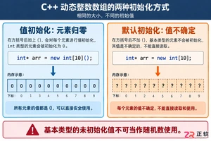
深入解析C++中动态数组的初始化机制,涵盖new操作符的不同用法、基本类型与类对象的初始化差异,以及为何在现代C++开发中应优先使用std::vector。
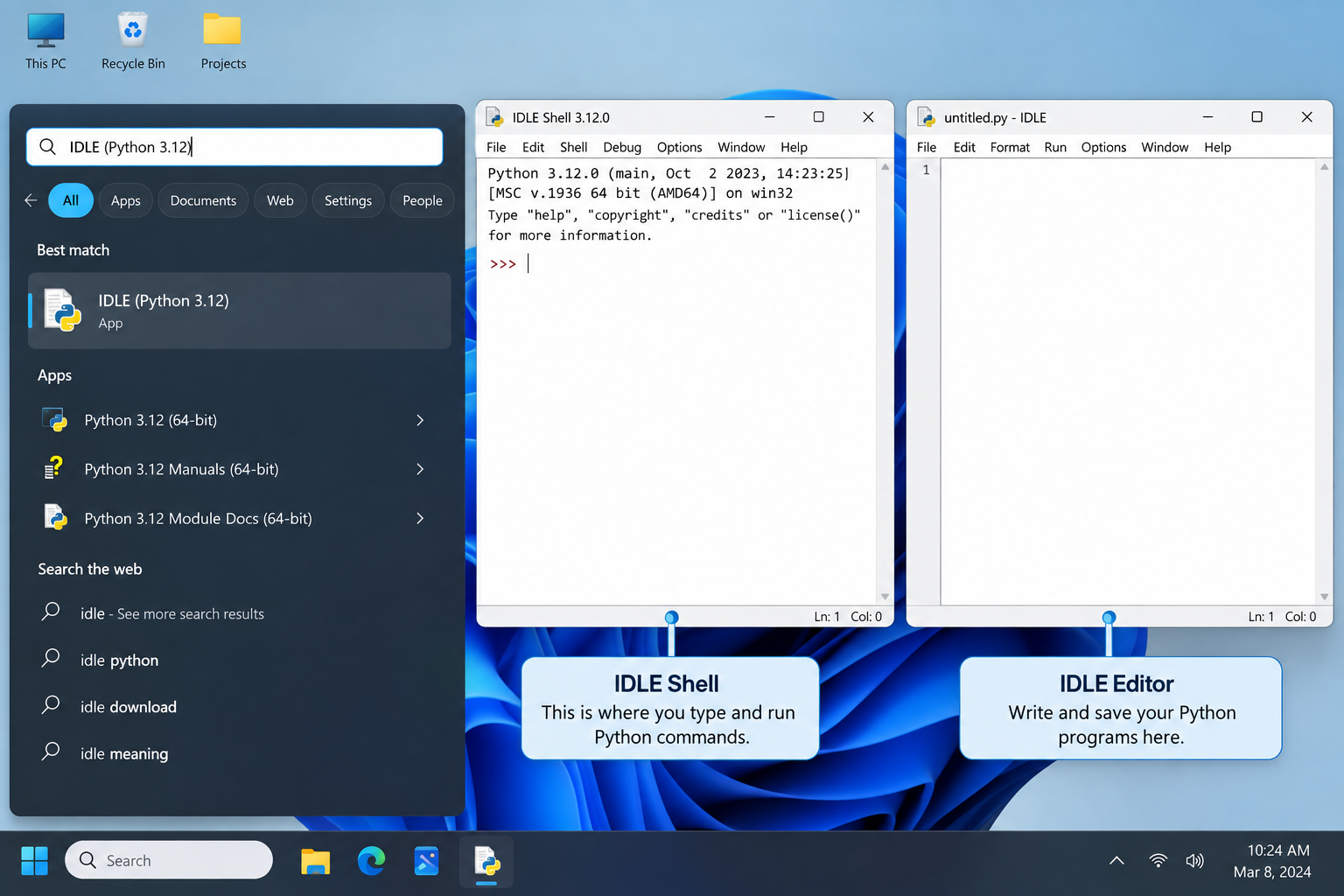
刚在Windows安装好Python却不知道如何启动?本文详细演示如何通过开始菜单找到并打开IDLE集成开发环境,以及如何在PowerShell或命令提示符中使用python和py命令启动交互式解释器、运行.py脚本文件。包含退出解释器的方法及常见启动问题排查,帮助初学者快速验证安装成功并开始编写代码。
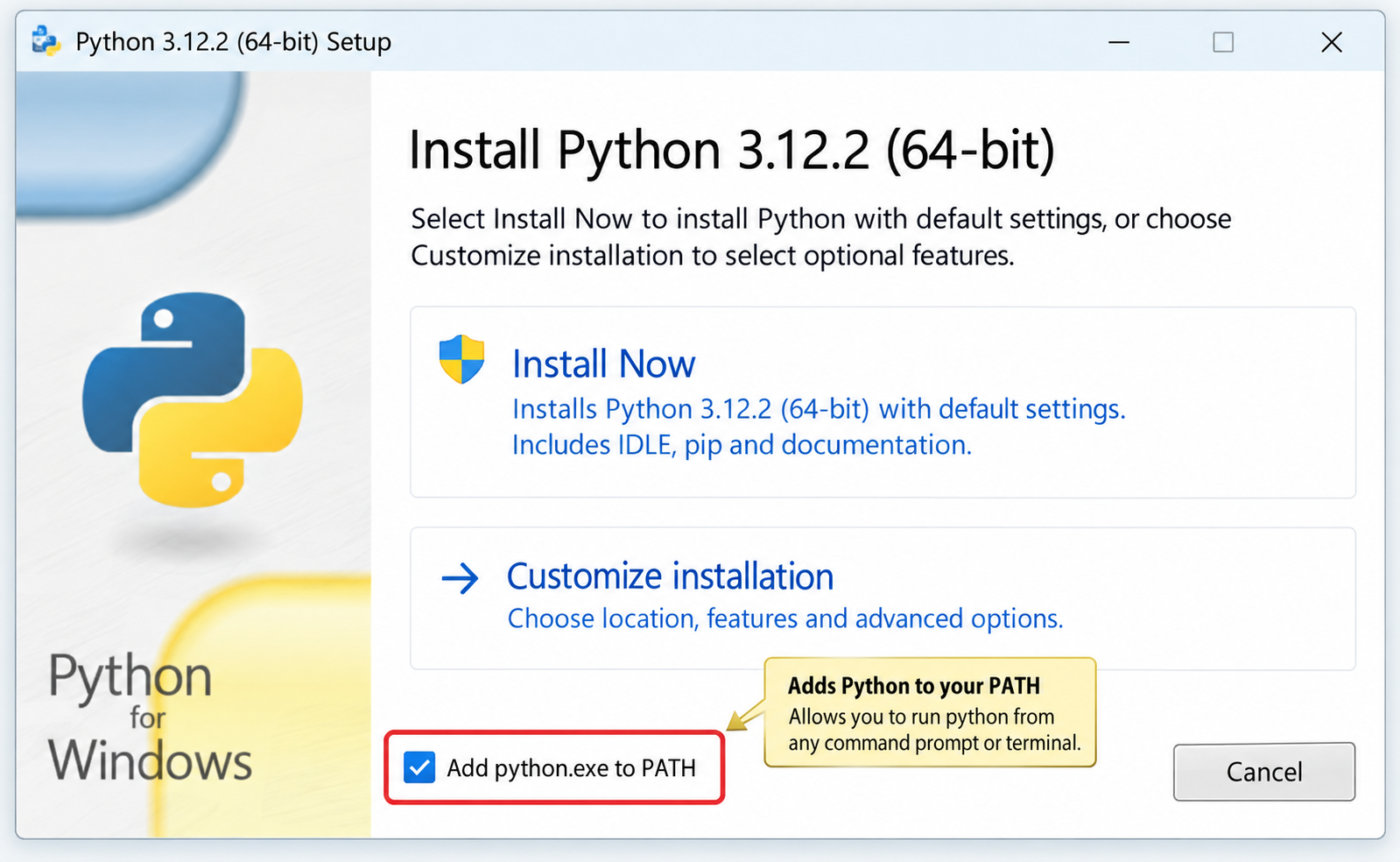
针对Windows初学者的Python安装实战指南。详细讲解如何从Python官网下载匹配架构的安装包,重点演示安装首屏勾选“Add python.exe to PATH”的关键操作,并提供使用python --version和py命令验证环境变量的具体步骤,帮助新手快速搭建开发环境并排查路径问题。

要想确认麒麟OS中Python程序的运行状态以及资源占用情况,我们可以这样做:用ps -ef | grep python来筛选进程;通过top命令,按P键排序查看实时负载;使用pgrep -f "script.py"精准获取PID;借助lsof -p PID验证文件打开状态。另外,还可以结合syst

在Debian系统上配置SSL证书通常涉及以下几个步骤:安装Web服务器:首先,你需要一个Web服务器,比如Apache或Nginx。这里以Apache为例。sudo apt updatesudo apt install apache2获取SSL证书:你可以从Let’s Encrypt免费获取SSL

要想让Python项目在统信UOS上正常运行,得先安装python3、python3-pip、python3-venv、python3-dev以及build-essential等组件。具体操作就是执行sudo apt install命令来一步到位完成安装,同时别忘了配置清华镜像源来给pip加速哦。在

在互联网上的各类网站中,无论大小,基本上都会有一个搜索框,用来给用户对内容进行搜索,小到站点搜索,大到搜索引擎搜索。从简单的来说,搜索功能确实很简单,一个简单的select语句就可以实现数据的搜索。而从复杂的来看,无论是搜索的精度还是搜索的效率,都是有很深的研究范围的。对于简单的搜索功能来说,一个s

立即在终端输入sudo shutdown -c取消倒计时关机,成功后显示“Shutdown cancelled”;若存在pmset重复任务,需再执行sudo pmset repeat cancel清除。Mac因Python脚本执行了os.system("sudo shutdown -h +10")或

之前写过一篇同步场景下用 Python 管理多个固定出口 IP 的实践(ExitPool + requests/httpx),覆盖了健康检查、故障转移和连接池复用。但在实际业务中,越来越多的场景用 asyncio 做高并发采集或批量接口调用——异步事件循环下多出口的管理方式和同步场景完全不同:单线程

写在前面:为什么静态出口 IP 不是"买了就行"不少团队在引入静态出口 IP 产品时,第一反应往往是:“地址配上去,这事就算完了。”可真到了真实业务里,静态出口 IP 真正能体现价值的地方,往往不在分配这一步,而在分配之后怎么管:地址有没有漂移,质量是否达标,某一条线路突然不可用时怎么切换,连接层又






Windows 10 是一款微软推出的经典操作系统,拥有硬件兼容性与多任务处理能力。它更偏向把系统状态查看和常用调节动作放在一起,适合需要持续观察和微调设备状态的场景。

极度公式是一款跨平台专业LaTeX公式识别编辑软件,支持OCR公式识别和多平台编辑。和使用说明,避免使用,享受完整功能与稳定支持。做扫描整理、文字提取和表格转换时,它能把识别后的处理步骤接得更顺,资料录入这类场景会省下不少时间。